How Facial Recognition Works – Part 1

(Update: part 2 of this post can be found here)

Facial recognition. What a hot topic this is today! Hardly a week goes by without it hitting the news in one way or another, and usually for the wrong reasons – i.e. privacy and its growing ubiquity. But have you ever wondered how this technology works? How is it that only now it has become such a hot topic of interest, whereas 10 years ago not many people cared about it at all?

In this blog post I hope to demystify facial recognition and present its general workings in a lucid way. I especially want to explain why it is that facial recognition has seen tremendous performance improvements over the last 5 or so years.

I will break this post up according to the steps taken in most facial recognition technologies and discuss each step one by one:

1. Face Detection and Aligning
2. Face Representation
3. Model Training
4. Recognition

(Note: in my next blog post I will describe Google’s FaceNet technology: the facial recognition algorithm behind much of the hype we are witnessing today.)

1. Face Detection and Aligning

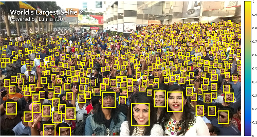
The first step in any (reputable) facial recognition technology is to detect the location of faces in an image/video. This step is called face detection and should not be confused with actual face recognition. Generally speaking, face detection is a much simpler task to facial recognition and in many ways it is considered a solved problem.

There are numerous face detection algorithms out there. A popular one, especially in the days when CPUs and memories weren’t what they are today, used to be the Viola-Jones algorithm because of its impressive speed. However, much more accurate algorithms have since been developed. This paper benchmarked a few of these under various conditions and the Tiny Faces Detector (published in the world-class Conference on Computer Vision and Pattern Recognition in 2017 – code can be downloaded here) came out on top:

If you wish to implement a face detection algorithm, here is a good article that shows how you can do this using Python and OpenCV. How face detection algorithms work, however, is beyond the scope of this article. Here, I would like to focus on actual face recognition and assume that faces have already been located on a given image.

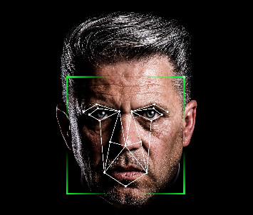
Once faces have been detected, the next (usual) step is to rotate and scale the face in order for its main features to be located in the same place, more or less, as the features of other detected faces. Ideally, you want the face to be looking directly at you with the lips and the position of the eyes parallel to the ground. The aligning of faces is an important step much akin to the cleaning of data (for those that work in data analysis). It makes further processing a lot easier to perform.

2. Face Representation

When we have a clean picture of a face, the next step is to extract a representation of it. A representation (often also called a signature) for a machine is a description/summary of a thing in a form that can be processed and analysed by it. For example, when dealing with faces, it is common to represent a face as a vector of numbers. The best way to explain this is with a simple example.

Suppose we choose to represent a face with a 2-dimensional vector: the first dimension represents the distance between the eyes, the second dimension the width of the nose. We have two people, Alice and Bob, and a photo of each of their faces. We detect and align the two faces in these photos and work out that the distance between the eyes of Alice is 12 pixels and that of Bob is 15 pixels. Similarly, the width of Alice’s nose is 4 pixels, Bob’s is 7 pixels. We therefore have the following representations of the two faces:

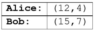
So, for example, Alice’s face is represented by the vector (12, 4) – the first dimension stores the distance between the eyes, the second dimension stores the width of the nose. Bob’s face is represented by the vector (15, 7).

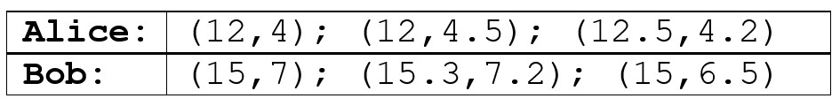
Of course, one photo of a person is not enough for a machine to get a robust representation/understanding of a person’s face. We need more examples. So, let’s say we grab 3 photos of each person and extract the representation from each of them. We might come up with the following list of vectors (remember this list as I’ll use these numbers later in the post to explain further concepts):

Having numbers like these to represent faces is much easier to deal with for a machine than raw pictures – machines are unlike us!

Now, in the above example, we used two dimensions to describe a face. We can easily increase the dimensionality of our representations to include even more features. For example, the third dimension could represent the colour of the eyes, the fourth dimension the colour of the skin – and so on. The more dimensions we choose to use to describe each face, generally speaking, the more precise our descriptions will be. And the more precise our descriptions are, the easier it will be for our machines to perform facial recognition. In today’s facial recognition algorithms, it is not uncommon to see vectors with 128+ dimensions.

Let’s talk about the facial features used in representations. The above example, where I chose the distance between the eyes and the width of the nose as features, is a VERY crude example. In reality, reputable facial recognition algorithms use “lower-level” features. For instance, in the late 1990s facial recognition algorithms were being published that considered the gradient direction (using Local Binary Patterns (LBP)) around each pixel on a face. That is, each pixel was analysed to see how much brighter or darker it was compared to its neighbouring pixels. Hence, brightness/darkness of pixels were the features chosen to create representations of faces. (You can see how this would work: each pixel location would have a relative different brightness/darkness score depending on a person’s facial structure).

Other lower-level features have been proposed for facial recognition algorithms, too. Some solutions, in fact used hybrid approaches – i.e. they used more than one low-level feature. There is an interesting paper from 2018 (M. Wang and W. Deng, “Deep Face Recognition: A Survey“, arXiv preprint) that summarises the history of facial recognition algorithms. This picture from the paper shows the evolution of features chosen for facial recognition:

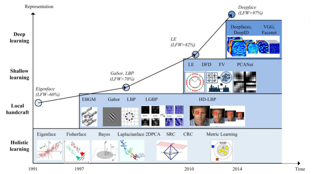
Notice how the accuracy of facial recognition algorithms (benchmarked on the LFW dataset) have increased over time depending on the type of representation used? Notice also the LBP algorithm, described above, making an appearance in the late 1990s? It gets an accuracy score of around 70%.

And what do you see at the very top of the graph? Deep Learning, of course! Deep Learning changed the face of Computer Vision and AI in general (as I discussed in this earlier post of mine). But how did it revolutionise facial recognition to the point that it is now achieving human-level precision? The key difference is that instead of choosing the features manually (aka “hand-crafting features” – i.e. when you say: “let’s use pixel brightness as a feature”), you let the machine decide which features should be used. In other words, the machine generates the representation itself. You build a neural network and train it to deliver vectors for you that describe faces. You can put any face through this network and you will get a vector out at the end.

But what does each dimension in the vector represent? Well, we don’t really know! We would have to break down the neural network used to see what is going on inside of it step by step. DeepFace, the algorithm developed by Facebook (you can see it mentioned in the graph above), churns out vectors with 128 dimensions. But considering that the neural network used has 120 million parameters, it’s probably infeasible to break it apart to see what each dimension in the vector represents exactly. The important thing, however, is that this strategy works! And it works exceptionally well.

3. Model Training

It’s time to move on to the next step: model training. This is the step where we train a classifier (an algorithm to classify things) on a list of face representations of people in order to be able to recognise more examples (representations) of these people’s faces.

Let’s go back to our example with our friends Alice and Bob to explain this step. Recall the table of six vector representations of their faces we came up with earlier? Well, those vectors can be plotted on a 2-dimensional graph like so:

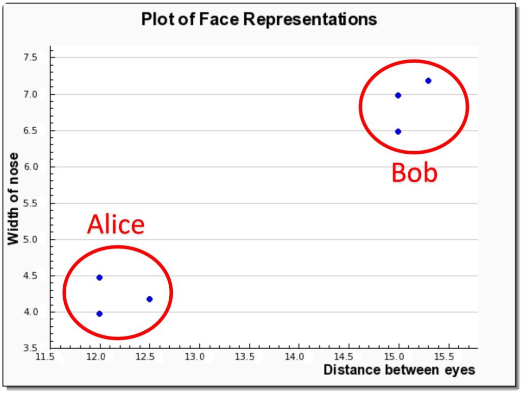
Notice how Alice and Bob’s representations cluster around each other (shown in red)? The bottom left data points belong to Alice, the top right belong to Bob. The job of a machine now will be to learn to differentiate between these two clusters. Typically, a well-known classification algorithm such as SVM is used for this.

If more than two clusters are present in the data (i.e. we’re dealing with more than two people in our data), the classifier will need to be able to deal with this. And then if we’re working in higher dimensions (e.g. 128+), the algorithm will need to operate in these dimensions, too.

4. Recognition

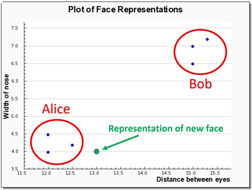
Recognition is the final step in the facial recognition process. Given a new image of a face, a representation will be generated for it, and the classification algorithm will provide a score of how close it is to its nearest cluster. If the score is high enough (according to some threshold) the face will be marked as recognised/identified.

So, in our example case, let’s say a new photo has emerged with a face on it. We would first generate a representation of it, e.g.: (13, 4). The classification algorithm will take this vector and see which cluster it lies closest to – in this case it will be Alice’s. Since this data point is very close to the cluster, a high recognition score will also be generated. The picture below illustrates this example:

This recognition step is usually extremely fast. And the accuracy of it is highly dependent on the preceding steps – the most important of which is the quality of the second step (the one that generates representations of faces).

Conclusion

In this post I described the major steps taken in a robust facial recognition algorithm. Each step was then described and an example use case was utilised to illustrate the concepts behind these steps. The major breakthrough in facial recognition came in 2014 when deep learning was used to generate representations of faces rather than the technique of hand-crafting features. As a result, facial recognition algorithms can now achieve near human-level precision.

(Update: part 2 of this post can be found here)

—

To be informed when new content like this is posted, subscribe to the mailing list:

Leave this field empty if you're human: