This post is the second post in my series on “How Facial Recognition Works”. In the first post I talked about the difference between face detection and face recognition, how machines represent (i.e. see) faces, how these representations are generated, and then what happens with them later for facial recognition to work.
Here, I would like to describe a specific facial recognition algorithm – one that changed things forever in this particular domain of artificial intelligence. The algorithm is called FaceNet and it was developed by Google in 2015.
FaceNet was published in a paper entitled “FaceNet: A Unified Embedding for Face Recognition and Clustering” at CVPR 2015 (a world-class conference for computer vision). When it was released it smashed the records of two top facial recognition academic datasets (Labeled Faces in the Wild and YouTube Faces DB) by a whopping 30% (on both datasets!). This is an utterly HUGE margin by which to defeat past state-of-the-art algorithms.
FaceNet’s major innovation lies in the fact that it developed a system that:
…directly learns a mapping from face images to a compact Euclidean space where distances directly correspond to a measure of face similarity. (Quote from original publication)
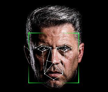
What this means is that it was the first algorithm to develop a deep neural network (DNN) whose sole task was to create embeddings for any face that was fed through it. That is, any image of a face inputted into the neural network would be given a 128-bit vector representation in the Euclidean space.
What this also means is that similar-looking faces are clustered/grouped together because they receive similar vector representations. Hence, clustering algorithms such as SVM or k-means clustering, can be employed on generated embeddings to perform facial recognition directly.
(To understand how such clustering algorithms work and to understand terms and concepts such as “embeddings” and “vector representations”, please refer to my first post on facial recognition where, as I have said earlier, I explain the fundamentals of facial recognition).
Another important contribution made in Google’s paper was its choice of method that it used to train the deep neural network to generate embeddings for faces. Usually, one would train a DNN for a fixed number of classes, e.g. 10 different types of objects to be detected in images. You would collect a large number of example images from each of these 10 different classes and tell the DNN during training which image contained which class. In tandem, you would use, for instance, a cross entropy loss function that would indicate to you the error rate of your model being trained – i.e. how far away you were from an “ideally” trained neural network. However, because the neural network is going to be used to generate embeddings (rather than, for example, to state whether there is a particular object out of 10 in an image), you don’t really know how many classes you are training your DNN for. It’s a different problem that you are trying to solve. You need a different loss function – something specific for generating embeddings. In this respect, Google decided to opt for the triplet-based loss function.
The idea behind the triplet-based loss function is to, during the training phase, take three example images from the training data:
- A random image of a person – we call this image the anchor image
- A random but different image of the same person – we call this image the positive image
- A random image of another person – we call this image the negative image.
During training, then, embeddings will be created for these three images and the triplet-based loss function’s task is to minimise the distance (in the Euclidean space) between the anchor and positive image and maximise the distance between the anchor and negative image. The following image from the original publication depicts this idea:
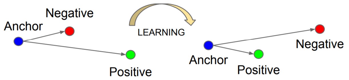
Notice the negative image initially is closer to the anchor than the positive image. The neural network would then go and adjust itself for the positive image to be closer to the anchor rather than the negative one. And the process would be repeated for different anchor, positive, and negative images.
Employing the triplet-based loss function to guide the training of the DNN was an incredibly intelligent move by Google. Likewise was the decision to decide to use a DNN to generate embeddings outright for faces. It really is no surprise that FaceNet busted onto the scene like it did and subsequently laid a solid foundation for facial recognition. The current state of this field owes an incredible amount to this particular publication.
If you would like to play around with FaceNet, take a look at its Github Repository here.
(Update: part 1 of this post can be found here)
—
To be informed when new content like this is posted, subscribe to the mailing list (or subscribe to my YouTube channel!):


Amar phone face lock nai