This post is another that has been inspired by a forum question: “What are some lesser known use cases for computer vision?” I jumped at the opportunity to answer this question because if there’s one thing I’m proud of with respect to this blog, it is the weird and wacky use cases that I have documented here.
Some things I’ve talked about include:
- Gait recognition as another form of biometric identification
- Lie detection from thermal imaging
- Extracting images from reflections in the eye
In this post I would like to add to the list above and discuss another lesser known use case for computer vision: heart rate estimation from colour cameras.
Vital Signal Estimation
Heart rate estimation belongs in the field called “Vital Signal Estimation” (VSE). In computer vision, VSE has been around for a while. One of the more famous attempts at this comes from 2012 from a paper entitled “Eulerian Video Magnification for Revealing Subtle Changes in the World” that was published at SIGGRAPH by MIT.
(Note: as I’ve mentioned in the past, SIGGRAPH, which stands for “Special Interest Group on Computer GRAPHics and Interactive Techniques”, is a world-renowned annual conference held for computer graphics researchers. But you do sometimes get papers from the world of computer vision being published there as is the case with this one.)
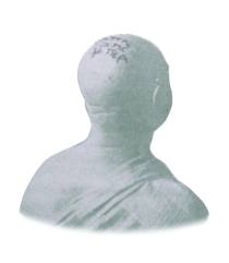
Basically, the way that VSE was implemented by MIT was that they analysed images captured from a camera for small illumination changes on a person’s face produced by varying amounts of blood flow to it. These changes were then magnified to make it easier to scrutinise. See, for example, this image from their paper:
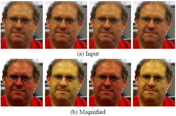
Amazing that these illumination changes can be extracted like this, isn’t it?
This video describes the Eulerian Video Magnification technique developed by these researchers (colour amplification begins at 1:25):
Interestingly, most research in VSE has focused around this idea of magnifying minute changes to estimate heart rates.
Uses of Heart Rate Estimation
What could heart rate estimation by computer vision be used for? Well, medical scenarios automatically come to mind because of the non-invasive (i.e. non-contact) feature of this technique. The video above (from 3:30) suggests using this technology for SIDS detection. Stress detection is also another use case. And what follows from this is lie detection. I’ve already written about lie detection using thermal imaging – here is one more way for us to be monitored unknowingly.
On the topic of being monitored, this paper suggests (using a slightly different technique of magnifying minute changes in blood flow to the face) detecting emotional reactions to TV programs and advertisements.
Ugh! It’s just what we need, isn’t it? More ways of being watched.
Making it Proprietary
From what I can see, VSE in computer vision is still mostly in the research domain. However, this research from Utah State University has recently been patented and a company called Photorithm Inc. formed around it. The company produces baby monitoring systems to detect abnormal breathing in sleeping infants. In fact, Forbes wrote an interesting article about this company this year. Among other things, the article talks about the reasons behind the push by the authors for this research and how the technology behind the application works. It’s a good read.
Here’s a video demonstrating how Photorithm’s product works:
Summary
This post talked about another lesser known use case of computer vision: heart rate estimation. MIT’s famous research from 2012 was briefly presented. This research used a technique of magnifying small changes in an input video for subsequent analysis. Magnifying small changes like this is how most VSE technologies in computer vision work today.
After this, a discussion of what heart rate estimation by computer vision could be used for followed. Finally, it was mentioned that VSE is still predominantly something in the research domain, although one company has recently appeared on the scene that sells baby monitoring systems to detect abnormal breathing in sleeping infants. The product being sold by this company uses computer vision techniques presented in this post.
To be informed when new content like this is posted, subscribe to the mailing list (or subscribe to my YouTube channel!):